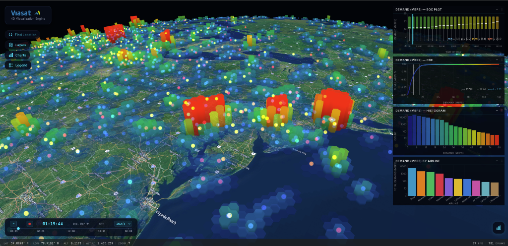
The hardest problem in geospatial visualization isn't rendering a map. It's animating a map through time — where every pixel, every hexagon, every track has a value that changes across hundreds or thousands of moments. The moment you add a temporal dimension to big geospatial data, every existing framework either collapses under the data volume, forces painful server-side infrastructure, or sacrifices interactivity for scale. Today we're open-sourcing Globe Trotter — a GPU-accelerated 4D globe engine and binary format architecture built from the ground up to make time a first-class dimension, at any scale, without servers. See who it's built for →
The Flex Format Architecture: GPU Zero-Copy Time Series
The reason Globe Trotter handles this scale at interactive frame rates is not clever rendering tricks — it's the Flex binary format architecture. Flex formats are the foundational data layer of the entire engine, and the foundation of a broader big data engineering platform. They are not compression wrappers around GeoJSON, nor are they tilesets generated by a tile server. They are GPU memory layouts — designed so that every byte of the file corresponds directly to a value that will be read by a GPU shader, with no intermediate parsing, transformation, or CPU-side data manipulation required.
Coming soon: Globe Trotter's visualization engine is the first component of a broader open-source Flex data engineering ecosystem — including a Rust SQL engine, a Python analytics SDK, and a streaming ingest pipeline — all built natively on the Flex formats. Watch this space.
What GPU Zero-Copy Means
Traditional geospatial formats — GeoJSON, Shapefiles, GeoPackage, even Parquet — are designed for interchange and analysis, not for GPU upload. Loading them into a WebGL or WebGPU pipeline requires a CPU-side parsing stage that extracts coordinates, builds index buffers, flattens nested structures, and marshals values into typed arrays before they can be uploaded to the GPU. For small datasets this is fine. For 1.47 million features across 1,440 time epochs, it's the bottleneck that makes interactive visualization impossible.
Flex formats eliminate this stage entirely. The pipeline is:
BigQuery / PostGIS
batch or streaming
static hosting
no parse
writeBuffer()
60 FPS
The Flex encoder runs when you generate your dataset — either as a one-time offline batch
job or a continuously running pipeline for datasets that update in real time. The resulting
binary file is then served from any
static host — a GCS bucket, S3, Azure Blob Storage, a CDN — and loaded directly into GPU
memory by the engine. There is no server-side rendering, no tile generation at query time,
and no CPU-side data processing in the browser. The CPU's only job is to call
writeBuffer().
This architecture also eliminates the traditional user-scaling bottleneck. Conventional geospatial platforms centralise work on the server: every concurrent user triggers a tile-render job, a database query, or a processing pipeline. That model caps out quickly — more users means more backend load, more infrastructure, and higher cost per viewer. By moving all computation to the encode step and serving static binary files from a CDN, Globe Trotter decouples viewer count from server load entirely. A visualisation that handles one user handles one million — the CDN absorbs the traffic and each viewer's GPU does the rendering independently. There is no query server to overload, no tile cache to warm, and no per-user cost to amortise.
The compression result: The mobile demand simulation dataset (1.47M hexagons × 1,440 epochs × 3 metrics) would be 87 GB as gzipped GeoJSON. In H3Flex format with sparse encoding and gzip compression it is 1.7 GB — a 51× reduction — and it requires zero CPU parsing to use.
Three Formats — One Architecture
Globe Trotter ships three Flex formats, each purpose-built for a different shape of geospatial time series data:
Pre-computed H3 hexagonal mesh with a temporal attribute tensor. Each hexagon stores a value per epoch per metric. The time dimension is stored in epoch-major order — a contiguous block of all hex values for epoch T, then T+1, enabling a WebGPU compute scatter to transition epochs in under 1ms regardless of grid size.
Data is sharded by metric: only the active metric's shard is in memory. Sparse and RLE encoding are auto-selected per shard. Each file is gzip-compressed.
1.47M hexagons 1,440 epochs sparse / RLE <200ms GPU upload
Points, lines, and polygons with epoch-major position arrays. Each
entity stores all of its positions across all time steps as a flat Float32 buffer.
The vertex shader reads two consecutive epoch positions and uses
mix() to interpolate — smooth sub-epoch animation at zero CPU cost.
Categorical attributes (airline, category, type) are dictionary-encoded and uploaded as a lookup texture — GPU categorical color mapping with no per-vertex branching.
83K tracks 1,440 epochs GPU interpolation 60 FPSGeometry-free columnar metric data for entity-level time series. Tracks a value per entity per epoch — e.g. per-airline demand across 1,440 minutes. Stored as a columnar Float32 tensor with dictionary-encoded string keys.
Powers the GPU chart system directly: histograms, time-series, and bar charts read from MetricFlex buffers already resident in GPU memory — no separate data fetch required.
columnar layout GPU charts dict encoding no geometryGenerating Flex Data — The Data SDK
Globe Trotter ships a Node.js data SDK with encoders for all three formats. Any source that can produce a row-oriented dataset — CSV, Parquet, BigQuery, PostGIS, a REST API — can be encoded into Flex format with a short script. The included mobile demand simulation generates a complete, realistic H3Flex + GeoFlex + MetricFlex dataset entirely from synthetic data, with no external dependencies:
import { H3FlexEncoder } from '@globe-trotter/data-sdk';

const encoder = new H3FlexEncoder({
  resolution: 5,          // H3 resolution (res-5 ≈ 252 km² cells)
  epochs:     1440,       // 24h at 1-minute resolution
  metrics:    ['demand_mbps', 'supply_mbps', 'utilization'],
  encoding:   'auto',     // sparse or RLE, chosen per shard
});

for (const row of rows) {
  encoder.add(row.h3index, row.epoch, row.metric, row.value);
}

await encoder.write('./public/data/demand.manifest.json');
// → demand.manifest.json + demand.shard.{metric}.h3f per metric
The encoder automatically selects sparse vs RLE encoding per shard based on value density, applies gzip compression, writes a manifest JSON that the engine uses for on-demand shard loading, and pre-computes the H3 mesh geometry so the engine never re-triangulates at runtime. For a 1.47M hexagon × 1,440-epoch × 3-metric dataset, the full encode runs in under two minutes on a laptop.
Coming soon: we will be open-sourcing PyFlex — a Python analytics SDK built on Rust (PyO3) with a Polars DataFrame interface, delivering a 20–40× performance gain over Pandas for Flex-scale temporal datasets.
Plugging Flex Into Your Visualization
Once your data is encoded, wiring it into a globe visualization requires only a YAML config update — no code:
basemap:
  style: satellite
  token: env:VITE_MAPBOX_TOKEN

camera:
  center: [39.0, -98.0]
  altitude: 12000

time:
  enabled: true
  speed: 60      # 1 real second = 60 simulated minutes
  loop:  true

layers:
  - name: Mobile Demand
    type: h3f-sharded
    url:  /data/demand.manifest.json
    metric: demand_mbps
    style:
      type:      ramp
      domain:    [0, 500]
      stops:     ["#0D1A80", "#1ABF59", "#F23319"]

  - name: Flight Tracks
    type: gfb
    url:  /data/flights.gfb
    style:
      type:      categorical
      attribute: airline
Why Scale Is the Differentiator
Most geospatial frameworks hit a hard wall around 10,000–50,000 GeoJSON features before frame rates drop below interactive thresholds. The community has developed workarounds — server-side tile generation, data aggregation on the fly, pre-rendered video — but each workaround reintroduces infrastructure complexity and sacrifices the key property that makes a visualization useful: the ability to interactively explore time.
| Approach | Temporal Interactivity | Scale Ceiling | Infrastructure |
|---|---|---|---|
| GeoJSON + Mapbox GL / Leaflet | Limited / custom code | ~10K features | Static hosting |
| deck.gl + tile server | Custom per-layer | Millions (tiled) | Tile server + DB |
| CesiumJS + CZML | Good for tracks | ~100K entities | Static or server |
| Kepler.gl | Good | Memory-limited | Static hosting |
| Globe Trotter + Flex | Full scrub/play/loop — built in | 1.5M+ features × 1,440 epochs | Static file hosting only |
Generate, Configure, Share
Globe Trotter collapses the entire workflow — from raw data to a shareable interactive globe — into three steps:
Generate Flex Data
Convert any source — CSV, Parquet, BigQuery, PostGIS, simulation output — into H3Flex, GeoFlex, or MetricFlex using the data SDK. Run it as a one-time batch job or continuously for real-time datasets.
Write a YAML Config
Define layers, styles, camera, time settings, and basemap in a single
globe-config.yaml. No JavaScript required.
Share a URL
Upload data + config to any static host. Send the URL. Your audience sees a live 4D globe — no install, no login.
Embed in Any Application
Globe Trotter ships as a framework-agnostic JavaScript library. The dist build is a single ES module — no dependencies, no peer packages — that drops into React, Vue, Angular, Svelte, or a plain HTML page without modification. The entire engine, rendering pipeline, and UI are contained in one import.
# npm / yarn / pnpm
npm install @globe-trotter/core
Initialising the engine takes three lines: create a canvas, instantiate the engine, load your config. Everything else — basemap, camera, time controls, layer rendering — is driven by the YAML config or the programmatic API.
import { GlobeTrotterEngine } from '@globe-trotter/core';

// Any <canvas> in your application — size it however you like.
const canvas = document.querySelector('#globe');

const engine = new GlobeTrotterEngine(canvas, {
  mapboxToken: import.meta.env.VITE_MAPBOX_TOKEN,
  basemap:     'satellite',
  autoStart:   true,
});

// Load layers, camera, and time from a YAML config …
await engine.loadConfig('/globe-config.yaml');

// … or drive it programmatically from your application state.
engine.setTime(epochSeconds);
engine.setMetric('demand_mbps');
Because the engine is just a class that wraps a <canvas>, it integrates
into component lifecycles naturally. In React, instantiate it in a
useEffect and call engine.dispose() on unmount. In Vue or
Angular, the pattern is identical. There is no virtual DOM involvement, no special
renderer, and no opinion about how your application manages state — the globe is a GPU
surface that responds to the method calls you make.
GPU Engine — Built to Feed the Flex Pipeline
The Flex architecture dictates the engine design. Because data arrives GPU-ready, the engine can focus entirely on rendering rather than data management:
Pure WebGPU, Zero Dependencies
Globe Trotter has no runtime dependencies — no Three.js, no Babylon.js,
no Mapbox GL renderer under the hood. Every GPU buffer, shader, and matrix multiply is
written from scratch. The globe, tiles, H3 layers, GFB tracks, and chart overlays all
render via WebGPU with WGSL compute shaders and instanced draws. WebGPU
is required; browsers without support receive a clear WebGPURequiredError.
Compute-First Rendering — Serving the Time Dimension
Every frame, the WebGPU pipeline runs compute before render. A
scatter compute shader reads the epoch index uniform and writes the
current epoch's hex values from a storage buffer into an R32F texture in
under 1ms — replacing what would be a 130ms CPU strip-upload loop in
WebGL2. The render pass then reads the texture directly. Epoch transitions are
imperceptible. A histogram compute shader bins 1.4M values via
atomicAdd
in <0.1ms, driving live GPU charts without blocking the main thread.
GPU Performance at Flex Scale
-
150× fewer tile draw calls — all visible satellite tiles render in a
single
drawIndexedInstanced()call via a 256-layer texture 2D array. - >100× faster epoch transitions — WebGPU compute scatter vs WebGL2 amortized strip upload (sub-1ms vs ~130ms).
-
~40× faster histogram computation — GPU
atomicAddbins 1.4M cells in <0.1ms vs ~4ms blocking CPU loop. - Zero per-frame GC pressure — pre-allocated scratch buffers for all uniform writes eliminate ~500 KB/s of garbage collection overhead.
GPU-Accelerated Chart System — Wired to Flex Data
Globe Trotter includes a full GPU-rendered chart system on a transparent WebGPU overlay canvas — no DOM elements, no Canvas2D, no external library. Six chart types are supported: histograms, heatmaps, CDFs, boxplots, bar charts, and time-series. Because chart data is read directly from MetricFlex buffers already in GPU memory, there is no separate data fetch for charts — they update in sync with the time scrubber automatically.
Agentic-First by Design
"Agentic-first" is not a feature added on top of Globe Trotter — it is the architectural philosophy that shaped every decision from day one. The entire codebase was vibe coded with Google Antigravity, Google's advanced agentic coding platform. Every line — the GPU engine, Flex format encoders, compute shaders, chart renderers, symbology dialogs, and all documentation — is AI-authored, Subject Matter Expert reviewed and verified. More importantly, Globe Trotter is designed to be operated by AI agents: from receiving a raw dataset and a natural-language description of what to visualise, through to encoding the data, writing the YAML config, and publishing a live interactive globe — with no human intervention required at any step.
The paradigm shift: Instead of an engineer spending days wrangling GeoJSON, configuring a tile server, and hand-writing visualisation code, an AI agent can ingest any standard geospatial format, generate production-quality Flex data, and publish a live 4D globe — in minutes, from a single natural language request.
Embedded Agent Skills
Globe Trotter ships with 10 embedded workspace agent skills, each one an invocable slash command. An AI agent working inside Globe Trotter loads complete expert knowledge for any subsystem on demand — without reading source code or documentation manually.
/globe-trotter-architecture
WebGPU render pipeline, compute shaders, instanced tile rendering, camera, time, filter engine, and WGSL shader conventions. Use when adding new renderer types or debugging frame rate issues.
/globe-trotter-yaml-config
Complete globe-config.yaml reference — all layer types, style specs,
camera, time, extrusion, basemap, charts, interaction popups, and UI widgets. Use when
configuring any layer or dataset.
/globe-trotter-styling
StyleEngine API — color ramps, categorical LUTs, opacity stops, compile/dispose lifecycle, GPU texture management, and the symbology dialog. Use when implementing custom color scales.
/globe-trotter-charting
GPU-accelerated chart system — heatmap, histogram, CDF, boxplot, barplot, and time-series chart types, shader architecture, and overlay system. Use when adding or modifying chart rendering.
/globe-trotter-data-pipeline
Data pipeline patterns for converting raw geospatial data into H3F, GFB, and MFB
formats using the @globe-trotter/data-sdk encoders. Use when onboarding
a new dataset.
/globe-trotter-bigquery-to-globe
End-to-end workflow: BigQuery SQL → H3Flex or GeoFlex → live globe layer. Use when visualising a BigQuery dataset on the globe from scratch.
/globe-trotter-custom-layers
Guide for creating custom renderer and layer types — WebGPU renderer contract, WGSL shaders, temporal interpolation, filter integration, and LayerManager registration.
/globe-trotter-deploy
Deployment patterns — static hosting, GKE, CDN, shard serving, Mapbox token management, and library builds. Use when deploying to production or configuring CDN caching.
/globe-trotter-performance
WebGPU profiling, GPU compute optimisations, memory budgeting, and scaling limits. Use when investigating low FPS or scaling to larger datasets.
/h3f-virtual-layers
Query-driven live H3 aggregation — mesh tile architecture, VirtualH3Loader pipeline, and YAML configuration. Use when adding virtual H3 layers that aggregate live data on demand.
Data Automation
Beyond development skills, Globe Trotter ships one end-to-end data automation pipeline that drives the full workflow from raw data to a live published globe:
/flex-create-dataset
Inspect source data, generate the correct Flex binary format, apply smart symbology,
and write the globe-config.yaml layer entry — end to end from a single
natural language description of the data.
Extend Globe Trotter Into Your Own Workflows
The skills and workflows architecture is an open extension point, not a closed system. Any
team that embeds Globe Trotter into a larger platform can add domain-specific skills and
workflows to the .agents/ directory — giving their own AI agents expert-level
knowledge of their specific datasets, naming conventions, deployment targets, and
organisational patterns. An agent working inside a telecommunications platform can load a
skill that knows that platform's H3 resolution choices, regional naming schema — and
invoke a workflow that re-encodes the latest epoch and pushes it to the CDN — without a
human in the loop. Globe Trotter's agentic architecture scales from a single developer
running a demo to a production platform where AI agents maintain a live global
visualisation system end to end.
Who Globe Trotter Is Built For
Globe Trotter addresses one underlying problem across many industries: large datasets where every measurement has a location and a timestamp, and the insight lies in watching the spatial picture change over time. The following matrix maps the roles and use cases where it delivers direct value.
Telecommunications & Network Engineering
| Role | Use Case |
|---|---|
| Network Planning Engineer | Visualise coverage, capacity, and demand across terrestrial radio networks (4G/5G/LEO) at global scale across time epochs |
| RF / Spectrum Analyst | Animate interference patterns, signal propagation, and spectrum utilisation across a full operational day |
| NOC / Operations Analyst | Live operational dashboard showing link states, faults, and traffic volumes across a global WAN |
| Capacity Planner | Model supply-vs-demand gaps across regions at per-minute resolution, identify under-served areas over time |
IoT & Sensor Networks
| Role | Use Case |
|---|---|
| IoT Platform Engineer | Real-time and historic visualisation of millions of device telemetry readings, spatially aggregated and animated across time |
| Industrial Asset Manager | Track fleet, equipment, or infrastructure health across a global footprint — surface anomalies by time and location |
| Smart City Analyst | Model sensor data (air quality, traffic, energy, water) across a city at per-minute resolution, replay events as animated H3 heatmaps |
| Supply Chain Analyst | Animate logistics flows, shipment positions, and delivery density across time to identify bottlenecks and demand spikes |
Remote Sensing & Earth Observation
| Role | Use Case |
|---|---|
| Satellite Data Scientist | Visualise raster-derived H3 outputs (NDVI, SAR coherence, SST, soil moisture) across temporal stacks without tile server infrastructure |
| Climate / Environmental Scientist | Animate decadal or multi-year geophysical datasets (sea level, ice extent, wildfire risk) at global scale with a shareable URL |
| Disaster Risk Analyst | Overlay multi-sensor event timelines — flood extent, fire perimeter, storm track — with underlying infrastructure and population data |
| EO Product Manager | Deliver client-facing interactive analytic outputs without provisioning tile or rendering servers |
Defence & Intelligence
| Role | Use Case |
|---|---|
| ISR Analyst | Temporal overlay of surveillance coverage, sensor dwell time, and event density across a geographic theatre |
| Mission Planning Analyst | Animate asset movements, coverage windows, and gap analysis across a planning timeline |
| Logistics / Readiness Officer | Track global asset posture, supply routes, and readiness metrics across time — surface degradation early |
Aviation, Logistics & Mobility
| Role | Use Case |
|---|---|
| ATM / Traffic Flow Manager | Animate flight track density, delay propagation, and sector loading across a full traffic day at continental scale |
| Airline Network Planner | Visualise route utilisation, OD demand, and schedule performance across a global network over time |
| Mobility Platform Analyst | Track ride-hail, micromobility, or autonomous vehicle fleet positions and trip density — replay demand patterns hour by hour |
Research & Academia
| Role | Use Case |
|---|---|
| Geospatial Data Scientist | Publish interactive spatio-temporal analyses as shareable URLs — no infrastructure budget, no license fees |
| Epidemiologist / Public Health Researcher | Animate disease incidence, intervention coverage, or mobility proxy data across time and geography |
| Urban Scientist | Model human activity patterns, land use change, or transport demand across cities across time at fine temporal resolution |